{waxer} makes the Wikimedia Analytics Query Service (AQS) REST API available and easy to use in R. With a consistent interface and output, {waxer} facilitates working with metrics & data available in AQS, especially when combined with modern data science frameworks like tidyverse for data wrangling.
Brief explanation of packages used: {purrr} makes it very easy to run multiple {waxer} queries programmatically, {dplyr} makes it easy to manipulate the obtained data, {lubridate} aids working with dates & times, and we use {ggplot2} for visualization. In some of these examples we will use purrr::map to apply a {waxer} function to a set of values we’re interested in while keeping all the other parameters constant. Here’s how map works:
fun <- function(a, b) {
  return(a + b)
}
map(-1:1, fun, b = 2)
#> [[1]]
#> [1] 1
#>
#> [[2]]
#> [1] 2
#>
#> [[3]]
#> [1] 3
Notice that the output is a list, which is map’s default behavior. We can also specify the output type by using the different flavors of map:
map_dbl(-1:1, fun, b = 2)
#> [1] 1 2 3
map_chr(-1:1, fun, b = 2)
#> [1] "1.000000" "2.000000" "3.000000"
Since the output of {waxer}’s API-querying functions is always a tibble (an extension of a data.frame), we will mostly be using the map_dfr function which stitches several tibbles into one (via dplyr::bind_rows).
Traffic-based data and metrics
Pageviews
This package uses the same API endpoint as the {pageviews} package for page view data. Similar to {pageviews}, the caveat is that the traffic data is only available from 1 August 2015. For legacy view counts, refer to {wikipediatrend} package.
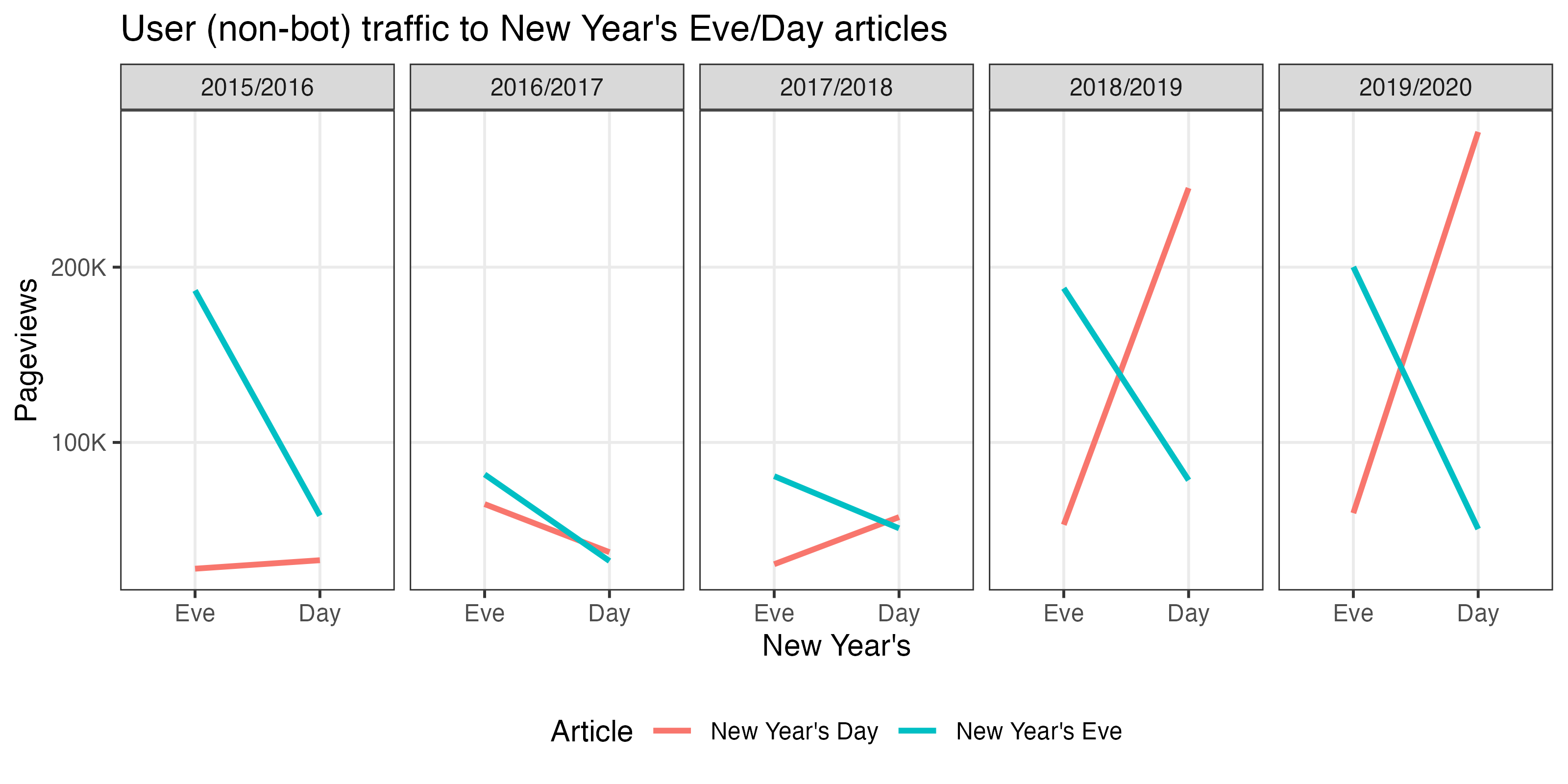
In this example we retrieve the page-views for the New Year’s Eve and New Year’s Day articles on English Wikipedia. Specifically, we’re interested in user traffic, which excludes known spiders/bots.
pageviews <- wx_page_views(
  project = "en.wikipedia",
  page_name = c("New Year's Eve", "New Year's Day"),
  access_method = "all",
  agent_type = "user",
  start_date = "20191231",
  end_date = "20200101"
)
pageviews
#> # A tibble: 4 x 4
#>   project      page_name      date        views
#>   <chr>        <chr>          <date>      <int>
#> 1 en.wikipedia New Year's Day 2019-12-31  59657
#> 2 en.wikipedia New Year's Day 2020-01-01 277191
#> 3 en.wikipedia New Year's Eve 2019-12-31 200158
#> 4 en.wikipedia New Year's Eve 2020-01-01  50580
In this case, the New Year’s Eve article was viewed much more on New Year’s Eve (December 31st) than on New Year’s Day. Similarly, the New Year’s Day article was viewed much more on New Year’s Day (January 1st) than on New Year’s Eve.
Work smarter, not harder
Now, suppose we wanted to see if this pattern is consistent across the years (starting with 2015/2016, since the API for pageviews starts from 2015-08-01). One way to do this would be to create start_date-end_date pairs across the years and use map2_dfr (not map_dfr) to iterate through the pairs:
new_years_dates <- tibble(
  start_date = as.Date("2015-12-31") + years(0:4),
  end_date = as.Date("2016-01-01") + years(0:4)
)
new_years_dates
#> # A tibble: 5 x 2
#>   start_date end_date
#>   <date>     <date>
#> 1 2015-12-31 2016-01-01
#> 2 2016-12-31 2017-01-01
#> 3 2017-12-31 2018-01-01
#> 4 2018-12-31 2019-01-01
#> 5 2019-12-31 2020-01-01
Notice that those are Dates, not “YYYYMMDD” strings. All of the start_date and end_date parameters in {waxer}’s functions accept either. This way we don’t have to use as.Date when we’re querying once and don’t have to use as.character on dates in situations like this.
new_years_views <- map2_dfr(
  new_years_dates$start_date,
  new_years_dates$end_date,
  wx_page_views,
  project = "en.wikipedia",
  page_name = c("New Year's Eve", "New Year's Day"),
  access_method = "all",
  agent_type = "user",
  granularity = "daily",
  .id = "pair"
)
head(new_years_views)
#> # A tibble: 6 x 5
#>   pair  project      page_name      date        views
#>   <chr> <chr>        <chr>          <date>      <int>
#> 1 1     en.wikipedia New Year's Day 2015-12-31  27956
#> 2 1     en.wikipedia New Year's Day 2016-01-01  32791
#> 3 1     en.wikipedia New Year's Eve 2015-12-31 186715
#> 4 1     en.wikipedia New Year's Eve 2016-01-01  58238
#> 5 2     en.wikipedia New Year's Day 2016-12-31  64817
#> 6 2     en.wikipedia New Year's Day 2017-01-01  37383
new_years_views <- new_years_views %>%
  mutate(
    pair = factor(
      new_years_views$pair, 1:5,
      paste(2015:2019, 2016:2020, sep = "/")
    ),
    day = case_when(
      month(date) == 12 & mday(date) == 31 ~ "Eve",
      month(date) == 1 & mday(date) == 1 ~ "Day"
    ),
    day = factor(day, c("Eve", "Day"))
  )
head(new_years_views)
#> # A tibble: 6 x 6
#>   pair      project      page_name      date        views day
#>   <fct>     <chr>        <chr>          <date>      <int> <fct>
#> 1 2015/2016 en.wikipedia New Year's Day 2015-12-31  27956 Eve
#> 2 2015/2016 en.wikipedia New Year's Day 2016-01-01  32791 Day
#> 3 2015/2016 en.wikipedia New Year's Eve 2015-12-31 186715 Eve
#> 4 2015/2016 en.wikipedia New Year's Eve 2016-01-01  58238 Day
#> 5 2016/2017 en.wikipedia New Year's Day 2016-12-31  64817 Eve
#> 6 2016/2017 en.wikipedia New Year's Day 2017-01-01  37383 Day

ggplot(new_years_views, aes(x = day, y = views)) +
  geom_line(aes(color = page_name, group = page_name), size = 1) +
  scale_y_continuous(
    minor_breaks = NULL,
    labels = scales::label_number(scale = 1e-3, suffix = "K")
  ) +
  facet_wrap(~ pair, nrow = 1) +
  labs(
    title = "User (non-bot) traffic to New Year's Eve/Day articles",
    color = "Article", x = "New Year's", y = "Pageviews"
  ) +
  theme_bw() +
  theme(legend.position = "bottom")
Including redirects
MediaWiki enables users to create redirects. This is usually done for common typos and aliases, to make it easier for users (both readers and editors) to arrive at a single article. The thing is, when someone visits a redirect page, that page view is not counted towards the total view count for the destination page. To include redirects in the output for wx_page_views:
pvs_with_redirects <- wx_page_views(
  "en.wikipedia",
  c("COVID-19 pandemic", "2019–20 coronavirus pandemic"),
  start_date = "20200401",
  end_date = "20200401",
  include_redirects = TRUE
)
Caution: this process requires finding all the redirects (within the article namespace) to the requested pages and retrieving those redirects’ page views. This has a considerable impact on the speed with which page views are retrieved. However, the function is optimized to work with many pages and will query the MediaWiki API the fewest times it can (since the redirects API supports up to 50 titles per query). Other than that the same rate limits apply.
head(pvs_with_redirects)
#> # A tibble: 6 x 5
#>   project     page_name             redirect_name              date        views
#>   <chr>       <chr>                 <chr>                      <date>      <int>
#> 1 en.wikiped… 2019–20 coronavirus … <NA>                       2020-04-01 810193
#> 2 en.wikiped… COVID-19 pandemic     <NA>                       2020-04-01    371
#> 3 en.wikiped… COVID-19 pandemic     2019-2020 China pneumonia… 2020-04-01     29
#> 4 en.wikiped… COVID-19 pandemic     2019-20 China pneumonia o… 2020-04-01     16
#> 5 en.wikiped… COVID-19 pandemic     China pneumonia outbreak   2020-04-01      4
#> 6 en.wikiped… COVID-19 pandemic     2019–20 China pneumonia o… 2020-04-01    153
On 1 April 2020, the 2019–20 coronavirus pandemic article had 96 redirects to it with traffic to them (at least 1 view). The most visited redirects are:
pvs_with_redirects %>%
  filter(!is.na(redirect_name)) %>%
  top_n(10, views) %>%
  select(redirect_name, views) %>%
  arrange(desc(views))
#> # A tibble: 10 x 2
#>    redirect_name                                      views
#>    <chr>                                              <int>
#>  1 2019–20 coronavirus pandemic                      810193
#>  2 2019–20 coronavirus outbreak                       40397
#>  3 2019–20 Wuhan coronavirus outbreak                 32575
#>  4 2019-20 coronavirus pandemic                        2741
#>  5 2019–20 outbreak of novel coronavirus (2019-nCoV)   2499
#>  6 2019–2020 coronavirus pandemic                      2496
#>  7 2020 coronavirus pandemic                           1707
#>  8 Coronavirus pandemic                                 895
#>  9 2020 coronavirus outbreak                            630
#> 10 COVID-19 outbreak                                    550
(The difference between the target article and a very similarly named redirect is that the actual article uses an en-dash but the redirect uses a minus sign, which is much more easily accessible on most keyboards than the more typographically-correct en-dash.)
If we wanted to roll up the page views to the redirects into the overall total for the article (and calculate some additional summary metrics), this is easily done within the tidyverse framework:
pvs_with_redirects %>%
  group_by(project, page_name, date) %>%
  summarize(
    total_views = sum(views),
    redirect_views = sum(views[!is.na(redirect_name)]),
    redirects = sum(!is.na(redirect_name))
  ) %>%
  ungroup
#> `summarise()` regrouping output by 'project', 'page_name' (override with `.groups` argument)
#> # A tibble: 2 x 6
#>   project    page_name           date       total_views redirect_views redirects
#>   <chr>      <chr>               <date>           <int>          <int>     <int>
#> 1 en.wikipe… 2019–20 coronaviru… 2020-04-01      810193              0         0
#> 2 en.wikipe… COVID-19 pandemic   2020-04-01      899025         898654        96
Project views
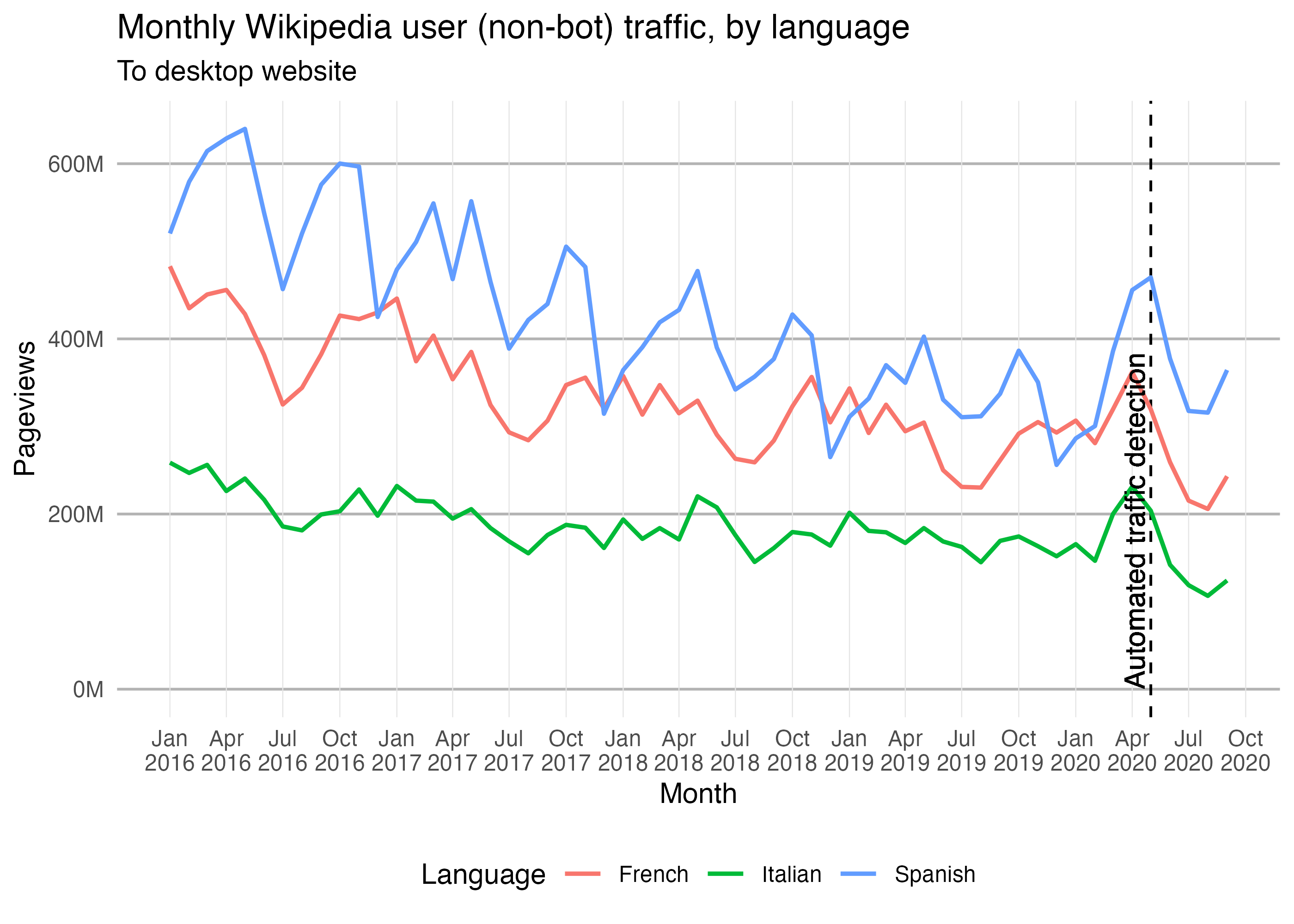
For consistency, the project parameter in every {waxer} function can only accept 1 value – unlike the page_name parameter in wx_page_views(). So if we want to get multiple projects’ views (the total number of page-views across all of the project’s pages), we can use the map_dfr to iterate through a named vector of projects, keeping all the other parameters the same:
projects <- c(
  "French" = "fr.wikipedia",
  "Italian" = "it.wikipedia",
  "Spanish" = "es.wikipedia"
)
project_views <- map_dfr(
  projects, wx_project_views,
  access_method = "desktop", agent_type = "user",
  granularity = "monthly", start_date = "20160101", end_date = "20201001",
  .id = "language"
)
head(project_views)
#> # A tibble: 6 x 4
#>   language project      date           views
#>   <chr>    <chr>        <date>         <int>
#> 1 French   fr.wikipedia 2016-01-01 482886364
#> 2 French   fr.wikipedia 2016-02-01 434907376
#> 3 French   fr.wikipedia 2016-03-01 450673104
#> 4 French   fr.wikipedia 2016-04-01 455875409
#> 5 French   fr.wikipedia 2016-05-01 428361642
#> 6 French   fr.wikipedia 2016-06-01 381467206
ggplot(project_views) +
  geom_vline(aes(xintercept = as.Date("2020-05-01")), linetype = "dashed") +
  geom_line(aes(x = date, y = views, color = language), size = 0.8) +
  geom_text(
    aes(
      x = as.Date("2020-05-01"), y = 0,
      label = "Automated traffic detection",
      vjust = "bottom", hjust = "left"
    ),
    angle = 90, nudge_x = -10
  ) +
  scale_y_continuous(
    minor_breaks = NULL,
    labels = scales::label_number(scale = 1e-6, suffix = "M")
  ) +
  scale_x_date(date_labels = "%b\n%Y", date_breaks = "3 month", minor_breaks = NULL) +
  labs(
    title = "Monthly Wikipedia user (non-bot) traffic, by language",
    subtitle = "To desktop website",
    x = "Month", y = "Pageviews", color = "Language"
  ) +
  theme_minimal() +
  theme(
    panel.grid.major.x = element_line(color = "gray90", size = 0.2),
    panel.grid.major.y = element_line(color = "gray70", size = 0.5),
    legend.position = "bottom"
  )
Hourly project views
We can also retrieve a project’s pageviews at an hourly granularity. For example:
hourly_views <- wx_project_views(
  "is.wikipedia",
  agent_type = "user",
  granularity = "hourly",
  start_date = "20191230",
  end_date = "20200102"
)
head(hourly_views)
#> # A tibble: 6 x 3
#>   project      time                views
#>   <chr>        <dttm>              <int>
#> 1 is.wikipedia 2019-12-30 00:00:00  1384
#> 2 is.wikipedia 2019-12-30 01:00:00   834
#> 3 is.wikipedia 2019-12-30 02:00:00   725
#> 4 is.wikipedia 2019-12-30 03:00:00   457
#> 5 is.wikipedia 2019-12-30 04:00:00   453
#> 6 is.wikipedia 2019-12-30 05:00:00   496
ggplot(hourly_views) +
  geom_line(aes(x = time, y = views)) +
  geom_vline(
    xintercept = lubridate::ymd(
      c("20191230", "20191231", "20200101", "20200102", "20200103"),
      tz = "UTC"
    ),
    linetype = "dashed"
  ) +
  scale_x_datetime(
    name = "Time",
    date_breaks = "6 hours", date_minor_breaks = "1 hour",
    date_labels = "%H:00\n%d %b"
  ) +
  scale_y_continuous(breaks = NULL, minor_breaks = NULL) +
  labs(
    title = "User (non-bot) traffic to Icelandic Wikipedia", y = NULL,
    subtitle = "Hourly pageviews around New Year's Eve 2019, New Year's Day 2020"
  ) +
  theme_minimal()
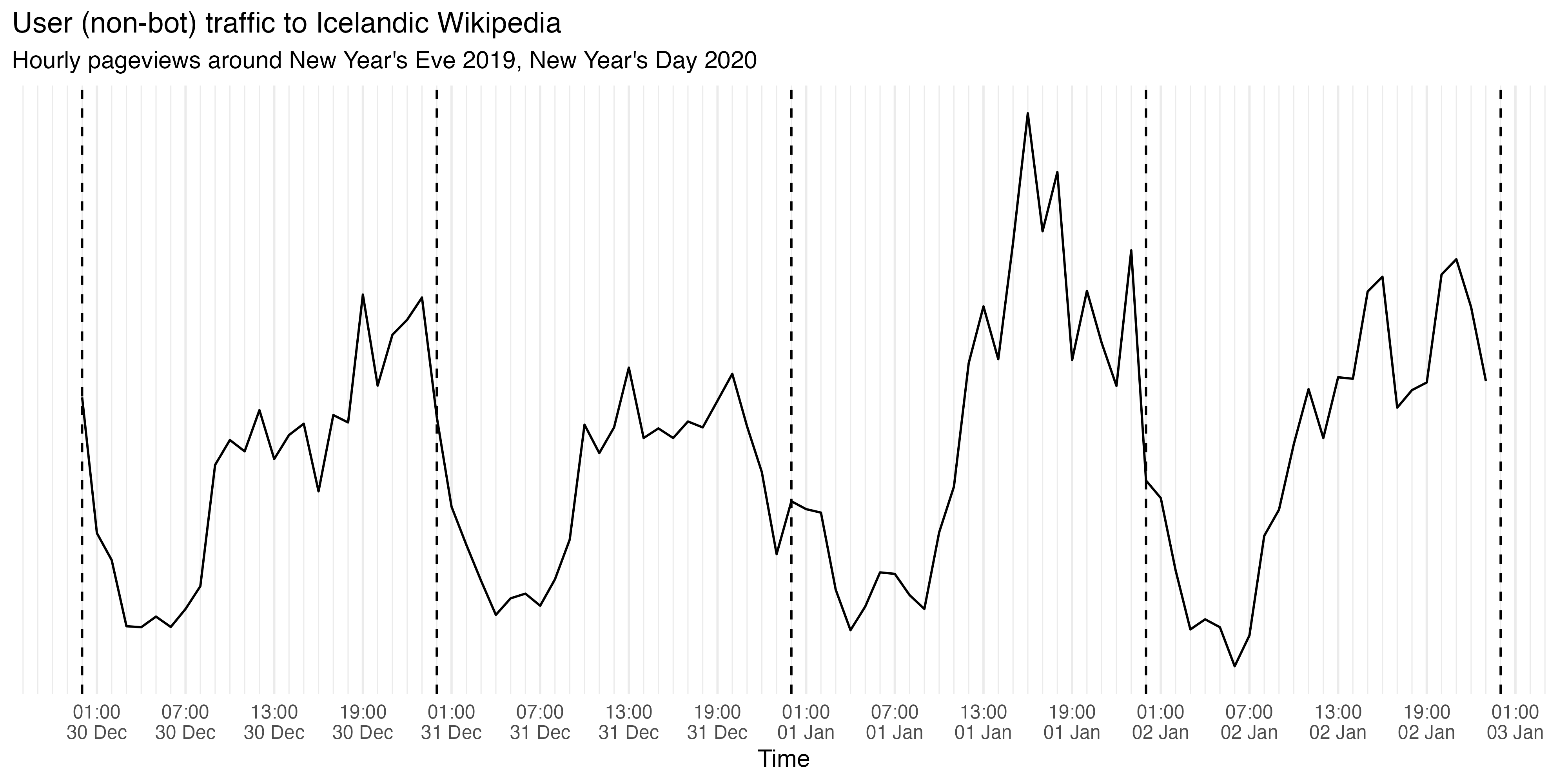
Compared to 11PM-12AM traffic on Dec 30th and January 1st, the 11PM-12AM traffic on Dec 31st is much lower. No surprises there since we would expect many Icelanders to be celebrating and partying around that time instead of reading/editing Wikipedia.
Top viewed articles
Top 1000 viewed articles each month from Jan 2019 to March 2019 on English Wikipedia:
top_viewed <- wx_top_viewed_pages(
  project = "en.wikipedia",
  granularity = "monthly",
  start_date = "20190101",
  end_date = "20190301"
)
Top 3 articles from each month:
top_viewed %>%
  # Exclude main page and other non-article pages:
  filter(page_name != "Main Page", !grepl("^(Special|Wikipedia)\\:.*", page_name)) %>%
  group_by(date) %>%
  top_n(3, views)
#> # A tibble: 9 x 5
#> # Groups:   date [3]
#>   date       project      page_name               views  rank
#>   <date>     <chr>        <chr>                   <int> <int>
#> 1 2019-01-01 en.wikipedia Ted Bundy             7293874     3
#> 2 2019-01-01 en.wikipedia Louis Tomlinson       5231127     4
#> 3 2019-01-01 en.wikipedia XHamster              4039614     6
#> 4 2019-02-01 en.wikipedia Freddie Mercury       6464633     3
#> 5 2019-02-01 en.wikipedia Louis Tomlinson       5497023     4
#> 6 2019-02-01 en.wikipedia Grover                4975383     5
#> 7 2019-03-01 en.wikipedia Captain Marvel (film) 7070703     3
#> 8 2019-03-01 en.wikipedia Luke Perry            6362644     4
#> 9 2019-03-01 en.wikipedia Us (2019 film)        4590483     6
Unique devices
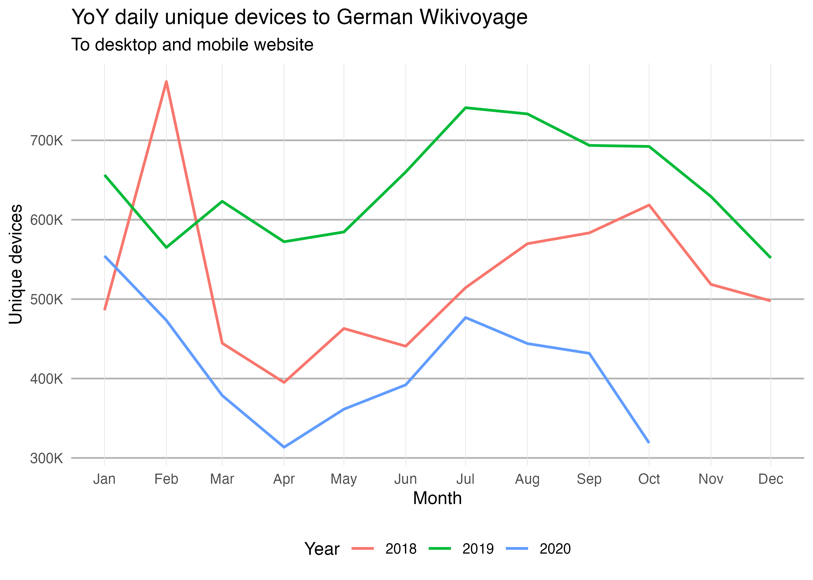
To obtain the monthly estimated number of unique devices that visited German Wikivoyage from Jan 2018 to June 2020:
unique_devices <- wx_unique_devices(
  project = "de.wikivoyage",
  granularity = "monthly",
  access_site = "all",
  start_date = "20180101",
  end_date = "20201031"
)
head(unique_devices)
#> # A tibble: 6 x 5
#>   project       date       devices offset underestimate
#>   <chr>         <date>       <int>  <int>         <int>
#> 1 de.wikivoyage 2018-01-01  486037 388266         97771
#> 2 de.wikivoyage 2018-02-01  773938 425827        348111
#> 3 de.wikivoyage 2018-03-01  444519 349013         95506
#> 4 de.wikivoyage 2018-04-01  395088 311396         83692
#> 5 de.wikivoyage 2018-05-01  463003 364774         98229
#> 6 de.wikivoyage 2018-06-01  440723 351782         88941
Which we can visualize with a periodicity plot:
unique_devices$year <- factor(year(unique_devices$date))
year(unique_devices$date) <- 2018

ggplot(unique_devices) +
  geom_line(aes(x = date, y = devices, color = year), size = 0.8) +
  scale_y_continuous(
    minor_breaks = NULL,
    labels = scales::label_number(scale = 1e-3, suffix = "K")
  ) +
  scale_x_date(date_labels = "%b", date_breaks = "1 month", minor_breaks = NULL) +
  labs(
    title = "YoY daily unique devices to German Wikivoyage",
    subtitle = "To desktop and mobile website",
    x = "Month", y = "Unique devices", color = "Year"
  ) +
  theme_minimal() +
  theme(
    panel.grid.major.x = element_line(color = "gray90", size = 0.2),
    panel.grid.major.y = element_line(color = "gray70", size = 0.5),
    legend.position = "bottom"
  )
User-based data and metrics
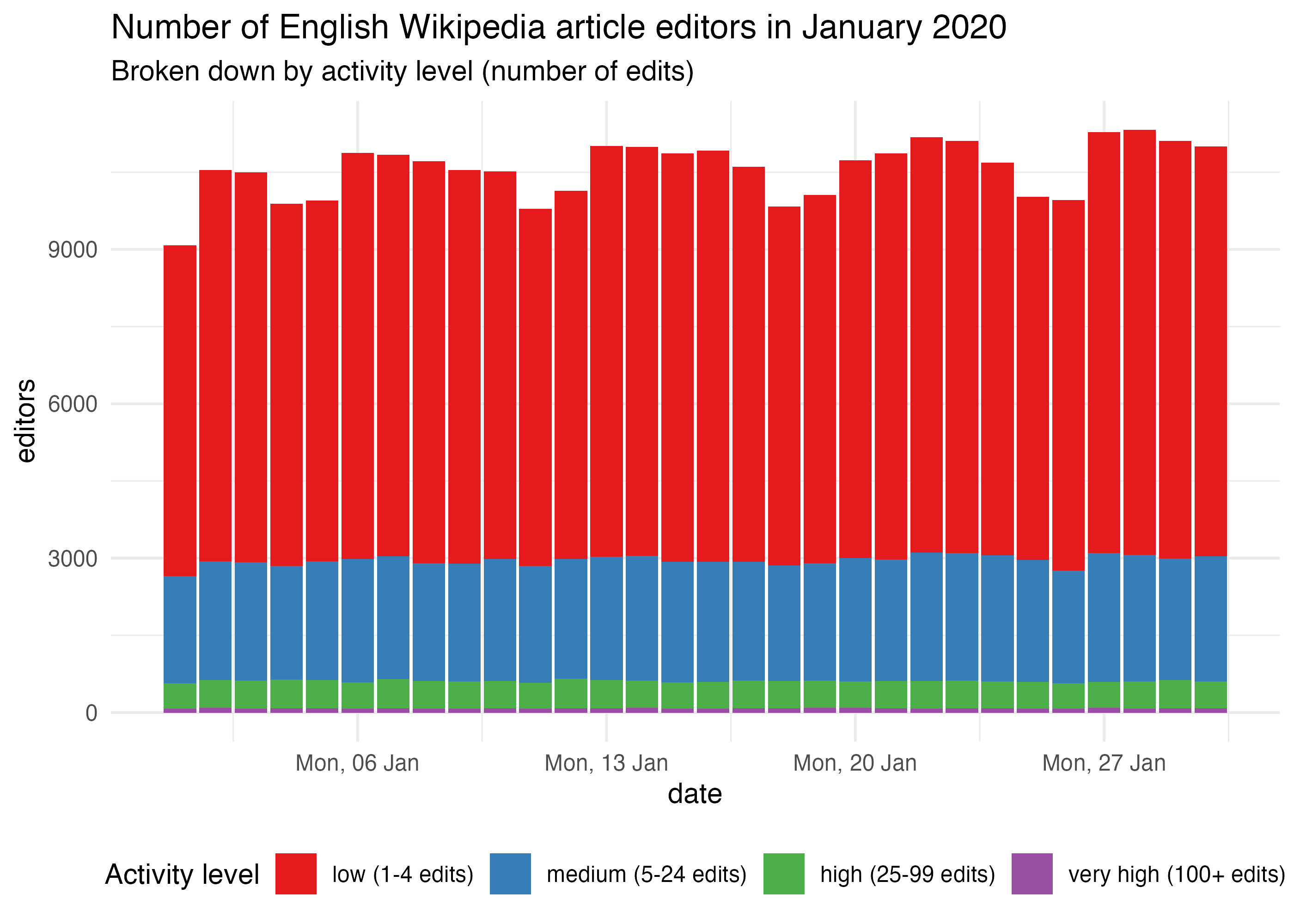
Suppose we wanted to get the daily number of non-bot active editors of content pages on English Wikipedia in January 2020. This is easy with {waxer}’s wx_active_editors function:
active_editors <- wx_active_editors(
  project = "en.wikipedia", editor_type = "user", page_type = "content",
  start_date = "20200101", end_date = "20200131"
)
head(active_editors)
#> # A tibble: 6 x 3
#>   project      date       editors
#>   <chr>        <date>       <int>
#> 1 en.wikipedia 2020-01-01    9072
#> 2 en.wikipedia 2020-01-02   10542
#> 3 en.wikipedia 2020-01-03   10495
#> 4 en.wikipedia 2020-01-04    9884
#> 5 en.wikipedia 2020-01-05    9950
#> 6 en.wikipedia 2020-01-06   10869
By activity level
Suppose we wanted to visualize these daily counts broken down by activity level:
activity_levels <- c(
  "low" = "1-4",
  "medium" = "5-24",
  "high" = "25-99",
  "very high" = "100+"
)
active_editors_by_activity <- map_dfr(
  activity_levels,
  wx_active_editors,
  project = "en.wikipedia", editor_type = "user", page_type = "content",
  start_date = "20200101", end_date = "20200131",
  .id = "activity_level"
)
head(active_editors_by_activity)
#> # A tibble: 6 x 4
#>   activity_level project      date       editors
#>   <chr>          <chr>        <date>       <int>
#> 1 low            en.wikipedia 2020-01-01    6425
#> 2 low            en.wikipedia 2020-01-02    7607
#> 3 low            en.wikipedia 2020-01-03    7581
#> 4 low            en.wikipedia 2020-01-04    7043
#> 5 low            en.wikipedia 2020-01-05    7015
#> 6 low            en.wikipedia 2020-01-06    7887
active_editors_by_activity <- active_editors_by_activity %>%
  mutate(
    activity_level = factor(
      activity_level,
      names(activity_levels),
      sprintf("%s (%s edits)", names(activity_levels), activity_levels)
    )
  )

ggplot(active_editors_by_activity, aes(x = date, y = editors)) +
  geom_col(aes(fill = activity_level)) +
  scale_x_date(date_labels = "%a, %d %b") +
  scale_fill_brewer("Activity level", palette = "Set1") +
  labs(
    title = "Number of English Wikipedia article editors in January 2020",
    subtitle = "Broken down by activity level (number of edits)"
  ) +
  theme_minimal() +
  theme(legend.position = "bottom")
By wiki
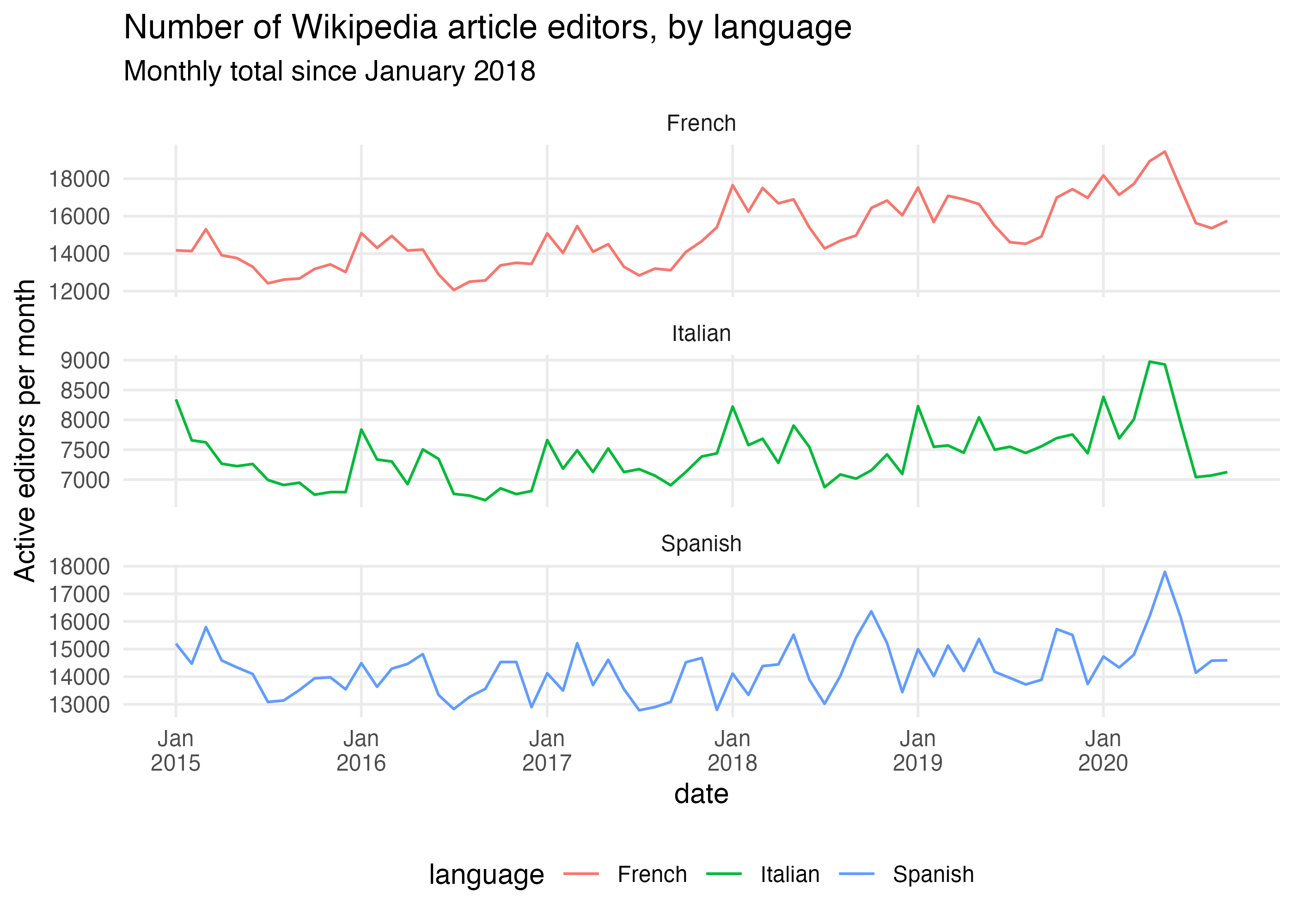
Similarly, we can obtain the (monthly) totals for several Wikipedias. This time we’re not breaking down by activity level (which is the default behavior for this function):
active_editors_by_wiki <- map_dfr(
  projects,
  wx_active_editors,
  editor_type = "user", page_type = "content",
  start_date = "20150101", end_date = "20201001",
  granularity = "monthly",
  .id = "language"
)
head(active_editors_by_wiki)
#> # A tibble: 6 x 4
#>   language project      date       editors
#>   <chr>    <chr>        <date>       <int>
#> 1 French   fr.wikipedia 2015-01-01   14175
#> 2 French   fr.wikipedia 2015-02-01   14138
#> 3 French   fr.wikipedia 2015-03-01   15304
#> 4 French   fr.wikipedia 2015-04-01   13911
#> 5 French   fr.wikipedia 2015-05-01   13764
#> 6 French   fr.wikipedia 2015-06-01   13302
ggplot(active_editors_by_wiki) +
  geom_line(aes(x = date, color = language, y = editors)) +
  scale_x_date(date_breaks = "1 year", minor_breaks = NULL, date_labels = "%b\n%Y") +
  scale_y_continuous(minor_breaks = NULL) +
  facet_wrap(~ language, ncol = 1, scales = "free_y") +
  labs(
    title = "Number of Wikipedia article editors, by language",
    subtitle = "Monthly total since January 2018",
    y = "Active editors per month"
  ) +
  theme_minimal() +
  theme(legend.position = "bottom")
Content-based data and metrics
Pages over time
How many new articles were created each month by registered users on Russian Wikipedia in December 2019?
new_pages <- wx_new_pages(
  "ru.wikipedia",
  editor_type = "user",
  page_type = "content",
  granularity = "monthly",
  start_date = "20191201",
  end_date = "20200101"
)
new_pages
#> # A tibble: 1 x 3
#>   project      date       new_pages
#>   <chr>        <date>         <int>
#> 1 ru.wikipedia 2019-12-01      5548
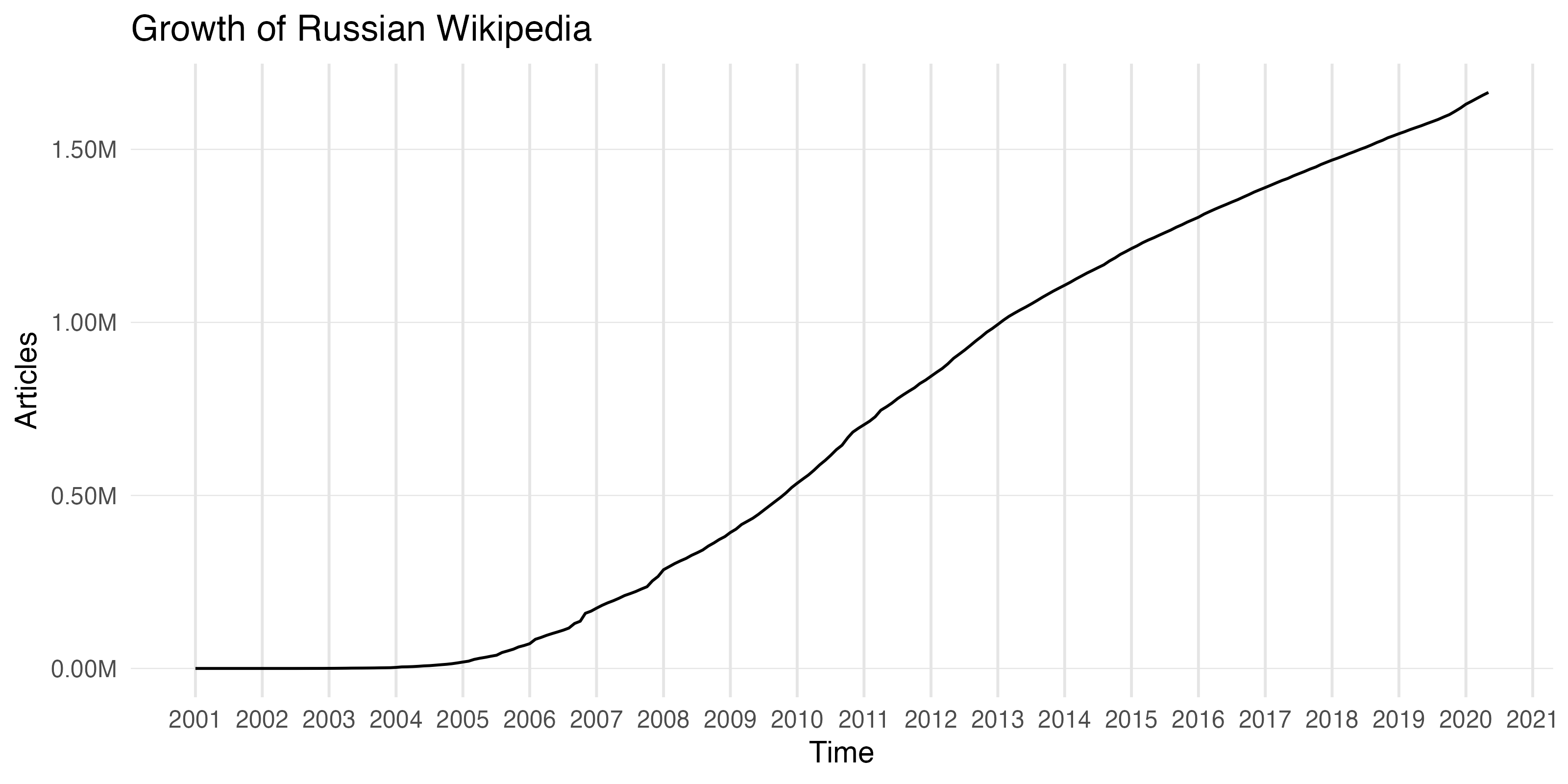
How has Russian Wikipedia grown over time since it started in May 2001?
total_pages <- wx_total_pages(
  "ru.wikipedia",
  editor_type = "all",
  page_type = "content", # focus on articles
  granularity = "monthly",
  start_date = "20010501",
  end_date = "20201001"
)
tail(total_pages)
#> # A tibble: 6 x 5
#>   project      date       total_pages existing_pages new_pages
#>   <chr>        <date>           <int>          <dbl>     <int>
#> 1 ru.wikipedia 2020-04-01     1619414        1609477      9937
#> 2 ru.wikipedia 2020-05-01     1630572        1619414     11158
#> 3 ru.wikipedia 2020-06-01     1639052        1630572      8480
#> 4 ru.wikipedia 2020-07-01     1647665        1639052      8613
#> 5 ru.wikipedia 2020-08-01     1656454        1647665      8789
#> 6 ru.wikipedia 2020-09-01     1664568        1656454      8114
ggplot(total_pages) +
  geom_line(aes(x = date, y = total_pages)) +
  scale_y_continuous(
    minor_breaks = NULL,
    labels = scales::label_number(scale = 1e-6, suffix = "M")
  ) +
  scale_x_date(date_labels = "%Y", date_breaks = "12 months", minor_breaks = NULL) +
  labs(
    title = "Growth of Russian Wikipedia",
    x = "Time", y = "Articles"
  ) +
  theme_minimal() +
  theme(
    panel.grid.major.y = element_line(color = "gray90", size = 0.2),
    panel.grid.major.x = element_line(color = "gray90", size = 0.5)
  )
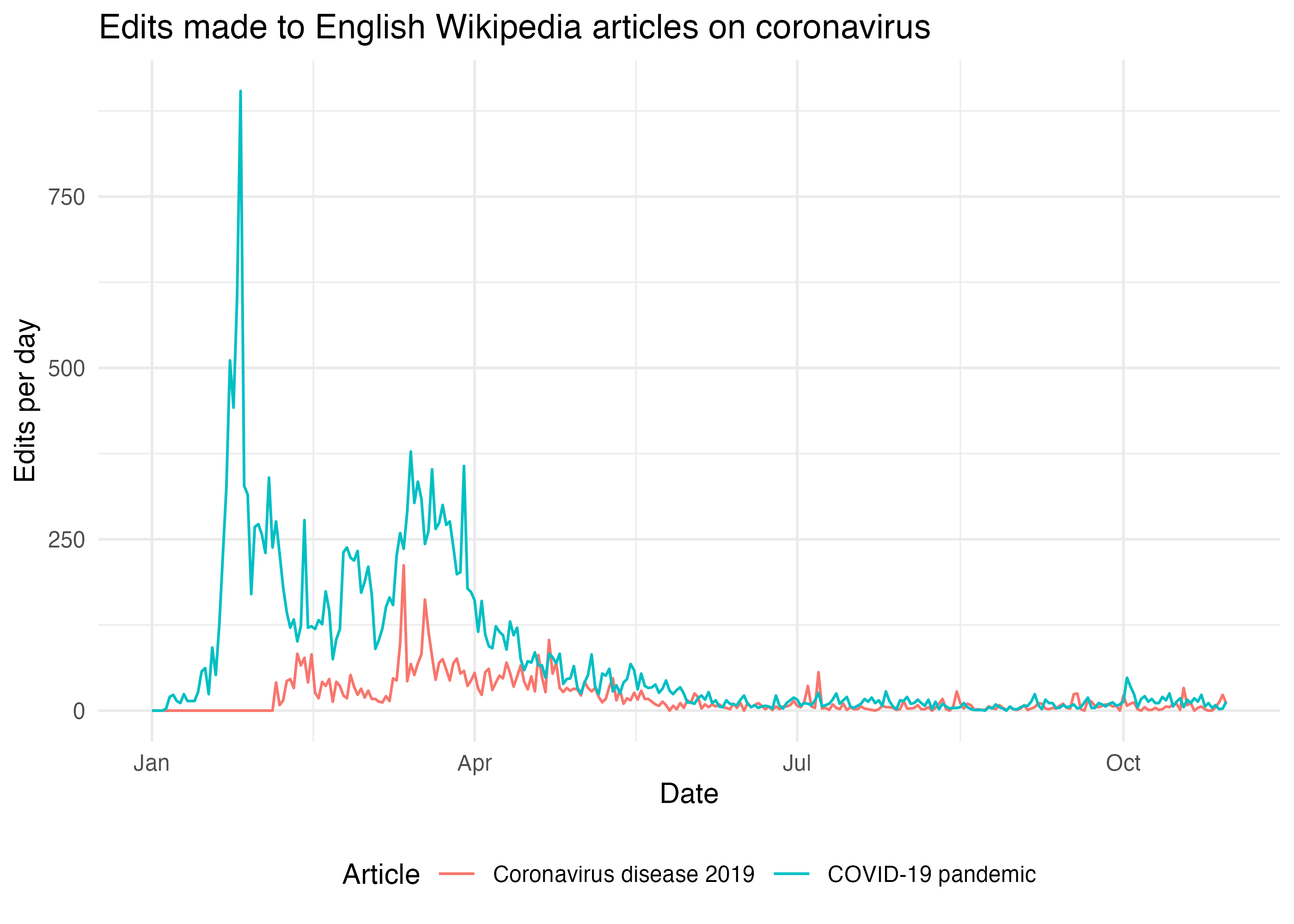
Edits to a page
page_edits <- wx_page_edits(
  "en.wikipedia",
  c("Coronavirus disease 2019", "COVID-19 pandemic"),
  start_date = "20200101",
  end_date = "20201031"
)
head(page_edits)
#> # A tibble: 6 x 4
#>   project      page_name                date       edits
#>   <chr>        <chr>                    <date>     <int>
#> 1 en.wikipedia Coronavirus disease 2019 2020-01-01     0
#> 2 en.wikipedia Coronavirus disease 2019 2020-01-02     0
#> 3 en.wikipedia Coronavirus disease 2019 2020-01-03     0
#> 4 en.wikipedia Coronavirus disease 2019 2020-01-04     0
#> 5 en.wikipedia Coronavirus disease 2019 2020-01-05     0
#> 6 en.wikipedia Coronavirus disease 2019 2020-01-06     0
ggplot(page_edits) +
  geom_line(aes(x = date, y = edits, color = page_name)) +
  labs(
    title = "Edits made to English Wikipedia articles on coronavirus",
    x = "Date", y = "Edits per day", color = "Article"
  ) +
  theme_minimal() +
  theme(legend.position = "bottom")
Editing activity
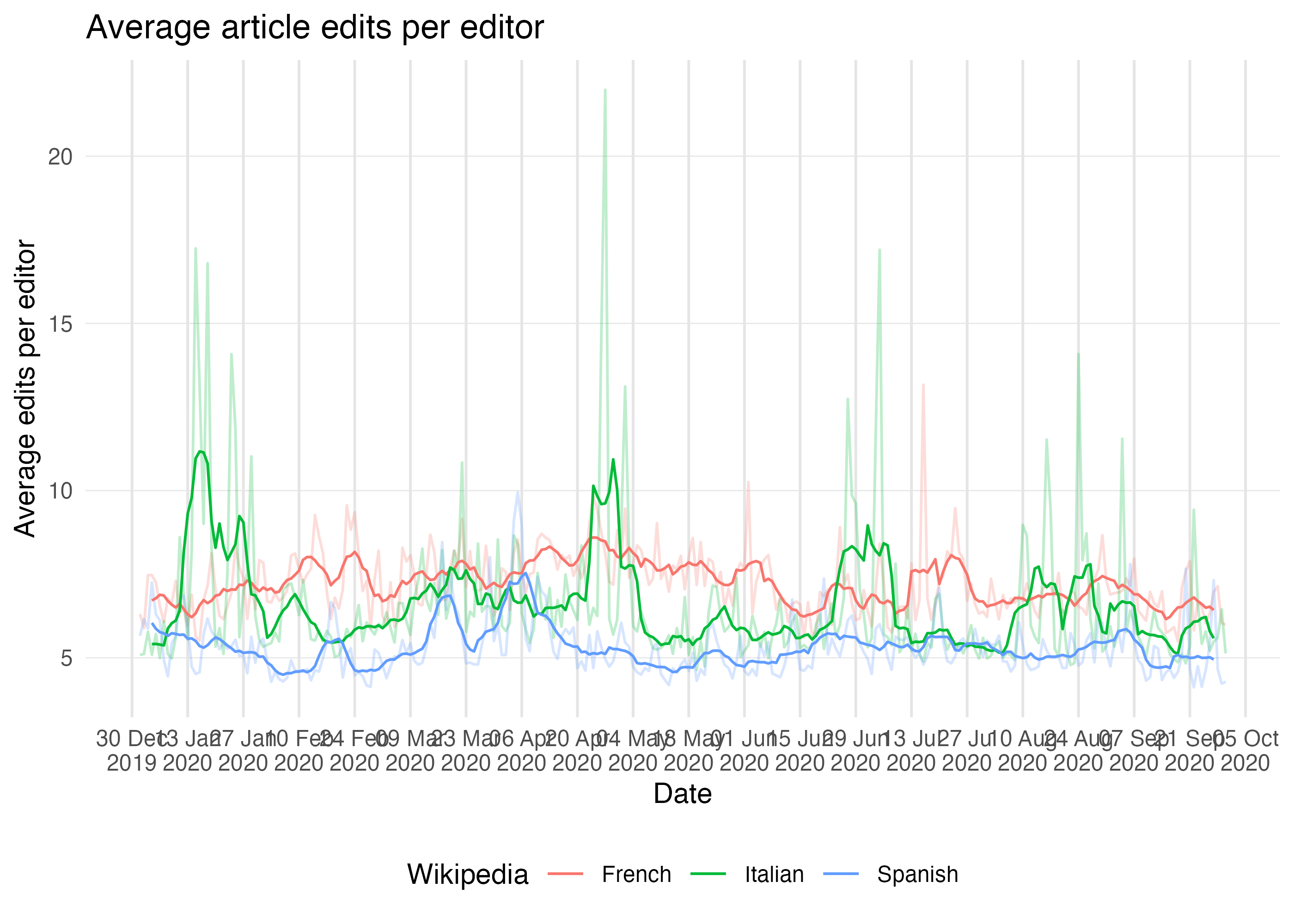
daily_edits <- map_dfr(
  projects,
  wx_project_edits,
  editor_type = "all", page_type = "content",
  start_date = "20200101", end_date = "20201001",
  granularity = "daily",
  .id = "language"
)
daily_editors <- map_dfr(
  projects,
  wx_active_editors,
  editor_type = "all", page_type = "content",
  start_date = "20200101", end_date = "20201001",
  granularity = "daily",
  .id = "language"
)
editing_activity <- daily_edits %>%
  left_join(daily_editors, by = c("project", "language", "date")) %>%
  mutate(edits_per_editor = edits / editors) %>%
  arrange(language, date)
head(editing_activity)
#> # A tibble: 6 x 6
#>   language project      date       edits editors edits_per_editor
#>   <chr>    <chr>        <date>     <int>   <int>            <dbl>
#> 1 French   fr.wikipedia 2020-01-01 17203    2724             6.32
#> 2 French   fr.wikipedia 2020-01-02 20693    3515             5.89
#> 3 French   fr.wikipedia 2020-01-03 26590    3558             7.47
#> 4 French   fr.wikipedia 2020-01-04 25138    3363             7.47
#> 5 French   fr.wikipedia 2020-01-05 26154    3605             7.25
#> 6 French   fr.wikipedia 2020-01-06 23235    3553             6.54
Using {RcppRoll} we can create a rolling 7-day average to smooth out the day-to-day variability, which will be helpful for visualization:
editing_activity %>%
  group_by(language) %>%
  mutate(
    rolling_avg = c(
      rep(NA, 3), # first 3 days
      RcppRoll::roll_mean(edits_per_editor, n = 7),
      rep(NA, 3) # last 3 days
    )
  ) %>%
  ungroup %>%
  ggplot(aes(x = date, color = language)) +
  geom_line(aes(y = edits_per_editor), alpha = 0.25) +
  geom_line(aes(y = rolling_avg)) +
  scale_y_continuous(minor_breaks = NULL) +
  scale_x_date(date_labels = "%d %b\n%Y", date_breaks = "2 weeks", minor_breaks = NULL) +
  labs(
    title = "Average article edits per editor",
    x = "Date", y = "Average edits per editor", color = "Wikipedia"
  ) +
  theme_minimal() +
  theme(
    panel.grid.major.y = element_line(color = "gray90", size = 0.2),
    panel.grid.major.x = element_line(color = "gray90", size = 0.5),
    legend.position = "bottom"
  )
#> Warning: Removed 18 row(s) containing missing values (geom_path).
Most edited pages
What were the top 5 most edited articles by on English Wikipedia from January through March of 2020?
edited_pages <- wx_top_edited_pages(
  "en.wikipedia",
  page_type = "content",
  granularity = "monthly",
  start_date = "20200101",
  end_date = "20200331"
)
head(edited_pages)
#> # A tibble: 6 x 5
#>   project      date       page_name                                  edits  rank
#>   <chr>        <date>     <chr>                                      <int> <int>
#> 1 en.wikipedia 2020-01-01 COVID-19 pandemic                           4943     1
#> 2 en.wikipedia 2020-01-01 Ukraine International Airlines Flight 752   2442     2
#> 3 en.wikipedia 2020-01-01 Deaths in 2020                              2185     3
#> 4 en.wikipedia 2020-01-01 Assassination of Qasem Soleimani            2145     4
#> 5 en.wikipedia 2020-01-01 2019–20 Australian bushfire season          1890     5
#> 6 en.wikipedia 2020-01-01 2020 Labour Party leadership election (UK)  1395     6
edited_pages %>%
  mutate(month = month(date, label = TRUE, abbr = FALSE)) %>%
  group_by(month) %>%
  top_n(5, desc(rank)) %>%
  select(month, rank, page_name)
#> # A tibble: 15 x 3
#> # Groups:   month [3]
#>    month     rank page_name
#>    <ord>    <int> <chr>
#>  1 January      1 COVID-19 pandemic
#>  2 January      2 Ukraine International Airlines Flight 752
#>  3 January      3 Deaths in 2020
#>  4 January      4 Assassination of Qasem Soleimani
#>  5 January      5 2019–20 Australian bushfire season
#>  6 February     1 COVID-19 pandemic
#>  7 February     2 COVID-19 pandemic by country and territory
#>  8 February     3 Deaths in 2020
#>  9 February     4 2020 Iowa Democratic presidential caucuses
#> 10 February     5 Timeline of the COVID-19 pandemic in February 2020
#> # … with 5 more rows